Sojourn (Dwell-Time) Analysis
The patch clamp recording technique can be used to measure the flow of current through a single ion channel in a patch of membrane, and hence the conductance of that channel. In many cases the conductance switches between two values - one high conductance and one low conductance, with no intermediary levels. In sojourn (dwell-time) kinetic analysis the information contained in the timing of these changes in conductance is used to deduce information about the molecular mechanisms that bring them about.
- Load the file agonist patch.
This is an event-only file showing the open- and closed-times of a simple 3-state agonist-activated model of the sort first proposed by del Castillo & Katz (1957). It was constructed from data simulated in Neurosim, with durations rounded to 0.01 ms and sojourns surrounding 0-duration sojourns merged. The transition equation is as follows:
\begin{equation} \ce{ Ag + R <=>[\ce{k_{+1} [Ag]}][\ce{k_{-1}}] Ag . R <=>[\beta][\alpha] Ag . R^*} \end{equation}where Ag is the agonist, R is the closed receptor-channel and R* is the open receptor-channel. In this model the channel gate cannot open until the agonist is bound, and the agonist cannot unbind when the gate is open. The simulation parameters were [Ag] = 1 mM, k+ = 100 mM-1s-1, k- = 500 s-1, β = 2000 s-1, α = 2000 s-1.
Inspection of the kinetic scheme reveals that there is just one open state (Ag.R*), with one transition path out of it, and therefore we would expect the open-time distribution to follow a single exponential. However, there are two closed states (closed-and-agonist-unbound Ag + R and closed-and-agonist-bound Ag.R) and the channel can switch between these two without opening. We would therefore expect the closed-time distribution to follow a double-exponential.
- Select the Event analyse: Sojourn analysis menu command to activate the Sojourn analysis dialog box.
The main display in this shows a histogram of either the Open time or Closed time durations, with options to Display it as either Normal, Ln Y, or Log X. The Normal display shows the count of sojourns in evenly-spaced time bins. The Ln Y display shows the natural log of the count, again in evenly spaced time bins. The default Log X display shows the square root of the count, in evenly-spaced logarithms of time. This display is usually thought to be the most appropriate for analysis of mixed exponentials, since each exponential component generates a peak in the histogram centred at the mean of that component (Sigworth & Sine, 1987).
A scaled pdf is drawn which by default shows a single exponential with a time constant of the mean sojourn duration. If you switch between the display options you will see that the open-time distribution is well-fitted by this default pdf.
- Now select Closed time in the Sojourn type group to display the closed time histogram.
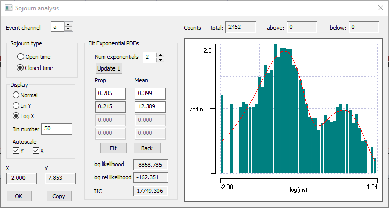
There are clearly two peaks on the Log X histogram. We would like to fit a mixture of two exponentials to this.
Fitting Mixed Exponentials
- In the Fit Exponential PDFs group, Increase the number of exponentials to 2.
If you hover the mouse in the general region of the histogram peaks, you will see X values of about -0.5 and 1.0. Remembering that these are log values, this suggests exponential means of about 0.3 and 10 respectively. Clearly, there are more elements in the shorter component (the peak is higher), but for simplicity let’s assume they have equal weighting. Also, the current mean of 0.5 is not too different from 0.3, so it does not need changing.
- Eenter 0.5 into the first proportion (note that the second proportion automatically adjusts to 0.5 so that the sum of proportions is 1).
- Leave the first mean at 0.5 and enter 10 as the value of the second mean.
You should see a 2-humped pdf which is very approximately fitting the histogram.
- Now click the Fit button. This uses Powell’s method to adjust the parameters of the exponential mixture to maximize the likelihood of the histogram. The pdf now fits rather well.

Note that fitting by maximum likelihood requires that you get the parameters approximately right before attempting to fit. If they are wildly wrong, the parameters are likely to head off in completely the wrong direction. Also note that sometimes you need to fit twice or three times, to get the best fit possible. Details about using the relative likelihood and BIC to judge the goodness-of-fit are given here.
The theoretical mean sojourns and proportions of a 3-state mechanism can be calculated analytically (Colquhoun & Hawkes, 1987), and in this case yield one component with a mean of 0.40 ms and a proportion of 0.786, and a second component with a mean of 12.6 ms and a proportion of 0.214 (1-p1). The fitted values are obviously rather nicely close to these values.